Applied Calibration Workflow

library(probcal)
library(dplyr)
#> 
#> Attaching package: 'dplyr'
#> The following objects are masked from 'package:stats':
#> 
#>     filter, lag
#> The following objects are masked from 'package:base':
#> 
#>     intersect, setdiff, setequal, union

Goal

This vignette shows a complete calibration workflow with a dataset included in R. The example uses iris as a binary classification problem: versicolor versus virginica.

The important point is the data split. The classifier is fitted on a training set. The calibrator is fitted on a calibration set. The final assessment uses a test set that was not used in either fitting step.

Prepare the data

set.seed(1001)
iris_binary <- iris |>
  filter(Species != "setosa") |>
  mutate(y = as.integer(Species == "virginica")) |>
  group_by(y) |>
  mutate(
    split = sample(rep(
      c("train", "calibration", "test"),
      times = c(25, 12, 13)
    ))
  ) |>
  ungroup()

iris_binary |>
  count(split, y)
#> # A tibble: 6 × 3
#>   split           y     n
#>   <chr>       <int> <int>
#> 1 calibration     0    12
#> 2 calibration     1    12
#> 3 test            0    13
#> 4 test            1    13
#> 5 train           0    25
#> 6 train           1    25

Fit a classifier

The classifier is deliberately simple. The goal is not to optimize predictive performance, but to produce probabilities that can be evaluated and calibrated.

train <- iris_binary |>
  filter(split == "train")

calibration <- iris_binary |>
  filter(split == "calibration")

test <- iris_binary |>
  filter(split == "test")

classifier <- glm(
  y ~ Sepal.Length + Sepal.Width,
  data = train,
  family = binomial()
)

calibration <- calibration |>
  mutate(raw_p = predict(classifier, calibration, type = "response"))

test <- test |>
  mutate(raw_p = predict(classifier, test, type = "response"))

Fit calibrators

Here we fit two calibrators on the calibration set. cal_beta() works directly on probabilities. cal_platt() can be used on raw probabilities or scores.

beta_fit <- cal_beta(calibration$raw_p, calibration$y)
platt_fit <- cal_platt(calibration$raw_p, calibration$y)

test <- test |>
  mutate(
    beta = predict(beta_fit, raw_p),
    platt = predict(platt_fit, raw_p)
  )

Compare calibration metrics

Calibration metrics are computed only on the test set.

metric_table <- bind_rows(
  test |>
    summarise(method = "raw", ece = ece(raw_p, y, bins = 5),
              mce = mce(raw_p, y, bins = 5), ace = ace(raw_p, y, bins = 5)),
  test |>
    summarise(method = "beta", ece = ece(beta, y, bins = 5),
              mce = mce(beta, y, bins = 5), ace = ace(beta, y, bins = 5)),
  test |>
    summarise(method = "platt", ece = ece(platt, y, bins = 5),
              mce = mce(platt, y, bins = 5), ace = ace(platt, y, bins = 5))
) |>
  mutate(across(where(is.numeric), function(x) round(x, 3)))

metric_table
#> # A tibble: 3 × 4
#>   method   ece   mce   ace
#>   <chr>  <dbl> <dbl> <dbl>
#> 1 raw    0.191 0.351 0.193
#> 2 beta   0.27  0.341 0.207
#> 3 platt  0.091 0.15  0.103

The best method is data dependent. A calibrator should be chosen on a validation criterion that matches the intended use of the probabilities.

Plot the calibrated probabilities

reliability_diagram(test$beta, test$y, bins = 5)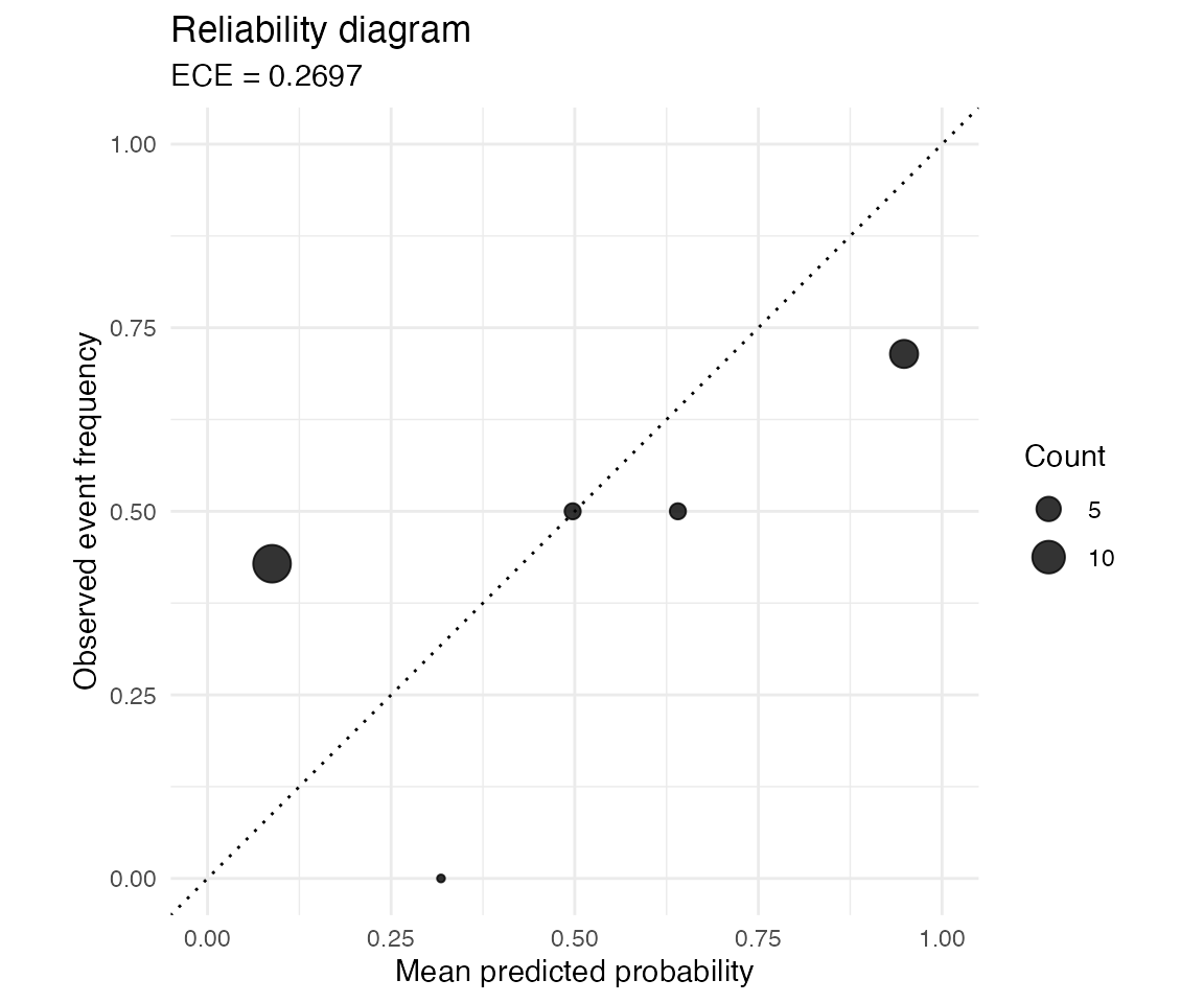

The diagonal represents perfect calibration. Points above the diagonal indicate bins where the observed event frequency is higher than the mean predicted probability. Points below the diagonal indicate overconfident predictions.