Calibrating Binary Probabilities

library(probcal)
library(dplyr)
#> 
#> Attaching package: 'dplyr'
#> The following objects are masked from 'package:stats':
#> 
#>     filter, lag
#> The following objects are masked from 'package:base':
#> 
#>     intersect, setdiff, setequal, union

Why calibration matters

A classifier can rank observations accurately while producing probabilities that are not calibrated. A probability of 0.8 is calibrated only if events with that prediction occur about 80 percent of the time. Calibration matters when a decision uses the numerical probability, for example in risk thresholds or cost sensitive decisions. It matters less when only the ranking is used.

A three-split workflow

Calibration should be fitted on data not used to train the classifier. A common workflow uses three parts: a model training set, a calibration set, and a test set. This vignette starts from already computed probabilities, so only the calibration and test split are shown.

set.seed(2026)
n <- 800
predictions <- data.frame(x = rnorm(n)) |>
  mutate(
    true_p = inv_logit(-0.5 + 1.2 * x),
    y = rbinom(n(), 1, true_p),
    raw_logits = 1.7 * (-0.5 + 1.2 * x),
    raw_p = inv_logit(raw_logits),
    split = sample(rep(c("calibration", "test"), each = n / 2))
  )

calibration <- predictions |>
  filter(split == "calibration")

test <- predictions |>
  filter(split == "test")

Fit a calibrator

Beta calibration works directly on probabilities. It is a useful default when the raw model probabilities show sigmoid-shaped miscalibration.

beta_fit <- cal_beta(calibration$raw_p, calibration$y)

test <- test |>
  mutate(beta = predict(beta_fit, raw_p))

test |>
  summarise(
    raw_ece = ece(raw_p, y, bins = 10),
    beta_ece = ece(beta, y, bins = 10)
  )
#>     raw_ece   beta_ece
#> 1 0.1044687 0.06968204

Compare methods

The package exposes the main binary calibration methods through the same fit-predict pattern.

platt_fit <- cal_platt(calibration$raw_p, calibration$y)
iso_fit <- cal_isotonic(calibration$raw_p, calibration$y)
hist_fit <- cal_histogram(calibration$raw_p, calibration$y, bins = 10)
temp_fit <- cal_temperature(calibration$raw_logits, calibration$y)

test <- test |>
  mutate(
    platt = predict(platt_fit, raw_p),
    isotonic = predict(iso_fit, raw_p),
    histogram = predict(hist_fit, raw_p),
    temperature = predict(temp_fit, raw_logits)
  )

bind_rows(
  test |> summarise(method = "raw", ece = ece(raw_p, y, bins = 10)),
  test |> summarise(method = "platt", ece = ece(platt, y, bins = 10)),
  test |> summarise(method = "beta", ece = ece(beta, y, bins = 10)),
  test |> summarise(method = "isotonic", ece = ece(isotonic, y, bins = 10)),
  test |> summarise(method = "histogram", ece = ece(histogram, y, bins = 10)),
  test |> summarise(method = "temperature", ece = ece(temperature, y, bins = 10))
) |>
  arrange(ece)
#>        method        ece
#> 1    isotonic 0.03805771
#> 2   histogram 0.05704115
#> 3        beta 0.06968204
#> 4       platt 0.07440266
#> 5 temperature 0.07679482
#> 6         raw 0.10446875

Reliability diagram

The reliability diagram shows calibration by bin. Points close to the diagonal have similar mean predicted probability and observed event frequency.

reliability_diagram(test$beta, test$y, bins = 10)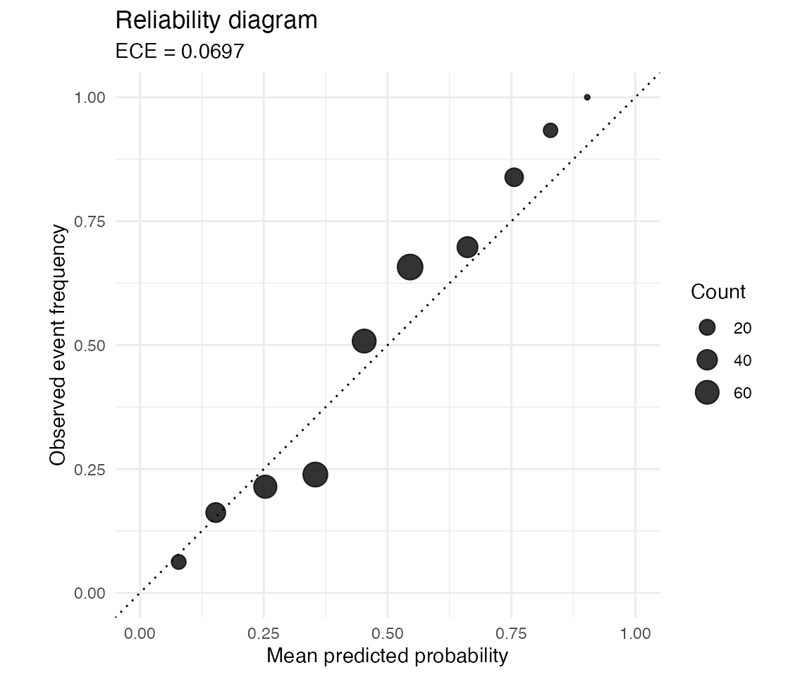

Cross-validated calibration

When the calibration set is small, cal_cv() produces out-of-fold calibrated probabilities while also fitting a final calibrator on all observations.

cv_fit <- cal_cv(
  predictions$raw_p,
  predictions$y,
  method = "histogram",
  folds = 5,
  bins = 10,
  seed = 1
)

predictions |>
  mutate(oof = cv_fit$oof_predictions) |>
  summarise(oof_ece = ece(oof, y, bins = 10))
#>      oof_ece
#> 1 0.04694437

Optional reference validation

The package includes optional tests that compare selected results against external reference implementations. These tests are not run for ordinary users unless the optional dependencies are installed.

Reference	What is compared	Package dependency
Python netcal	ece(), mce(), ace()	reticulate and Python netcal
Python netcal	cal_histogram() with equal-width bins	reticulate and Python netcal
R betacal	cal_beta() predictions	betacal

This keeps the runtime package in R while still allowing numerical checks against the reference implementation during development.

Current scope

The current scope covers binary and multiclass probability calibration for predictions that were already produced by another model. Neural calibration, Bayesian binning, and direct integration with model-training frameworks are not part of the package interface.