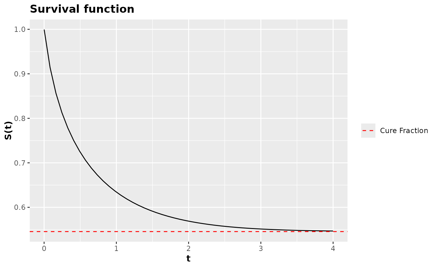
Numerical survival function

Constructs the numerical survival function from a probability density function.

Usage

survival_function(pdf)

Arguments

pdf: The probability density function.

Value

Returns the numerical value of survival at time \(t\).

Details

The function survival_function() returns a function in terms of \(t\) and the additional parameters of the probability density function that is passed as an argument to pdf. The returned function calculates survival numerically, making the implementation of survival functions quick. The returned function is vectorized in \(t\), that is, a vector of time instances can be passed as an argument.

The survival function returned by survival_function() also has a t0 argument that defaults to t0 = 0. The t0 argument is the initial time for the calculation of the survival function. The t0 argument is useful for calculating the survival function from a start time different from zero. In most cases, you should not change the default value of t0.

The function returned by survival_function() also has the argument asymptotic_quantile = 30, which defaults to 30. This argument is responsible for evaluating the survival function at the 30th quantile, providing a good approximation for the cure fraction. As this is a numerical evaluation, and depending on the complexity of the base probability density function, it may be that asymptotic_quantile = 30 produces an error, requiring the value of asymptotic_quantile to be changed.

References

NADARAJAH, Saralees; KOTZ, Samuel. The beta exponential distribution. Reliability engineering & system safety, v. 91, n. 6, p. 689-697, 2006.

Examples

survival_weibull <- survival_function(dweibull)
survival_weibull(0:10, shape = 2, scale = 1, asymptotic_quantile = 30)
#>  [1] 1.000000e+00 3.678794e-01 1.831564e-02 1.234098e-04 1.125352e-07
#>  [6] 1.392675e-11 0.000000e+00 1.110223e-16 0.000000e+00 5.218048e-15
#> [11] 3.885781e-14
#> attr(,"time")
#>  [1]  0  1  2  3  4  5  6  7  8  9 10
#> attr(,"cure_fraction")
#> [1] 0
#> attr(,"class")
#> [1] "survival_function"

# The user can also define any density
# Saraless Nadarajah and Samnuel Kotz (2006)
beta_exponential <- function(x, a, b, lambda){
 lambda / beta(a, b) * exp(-b * lambda * x) * (1 - exp(-lambda * x))^(a - 1)
}
survival_beta_exponential <- survival_function(beta_exponential)
survival_beta_exponential(
  t = seq(0.01, 1.5, length.out = 20L),
  a = 1.5,
  b = 1.8,
  lambda = 1.5
)
#>  [1] 0.99609097 0.91082931 0.79861387 0.68589560 0.58145868 0.48847323
#>  [7] 0.40762323 0.33841738 0.27983026 0.23063664 0.18958810 0.15550403
#> [13] 0.12731374 0.10407270 0.08496250 0.06928346 0.05644330 0.04594448
#> [19] 0.03737152 0.03037915
#> attr(,"time")
#>  [1] 0.01000000 0.08842105 0.16684211 0.24526316 0.32368421 0.40210526
#>  [7] 0.48052632 0.55894737 0.63736842 0.71578947 0.79421053 0.87263158
#> [13] 0.95105263 1.02947368 1.10789474 1.18631579 1.26473684 1.34315789
#> [19] 1.42157895 1.50000000
#> attr(,"cure_fraction")
#> [1] 4.893063e-08
#> attr(,"class")
#> [1] "survival_function"

# Sobrevivencia do modelo de fragilidade descreta ZMPG
fragility_model <- pdf_fragility_zmpg(pdf = dweibull)
fragility_survival <- survival_function(fragility_model)
fragility_survival(
  t = seq(0.001, 4, length.out = 50L),
  shape = 1.3,
  scale = 1.2,
  mu = 3.7,
  rho = 1.5,
  phi = 2.5,
  asymptotic_quantile = 30
 ) |> plot()