Inspecting the theoretical density with the base density

Inspect the probability density function used as the base with the theoretical density function from which observations are desired.

Usage

inspect(
  f,
  args_f,
  f_base,
  args_f_base,
  xlim,
  c = 1,
  alpha = 0.4,
  color_intersection = "#BB9FC9",
  color_f = "#F890C2",
  color_f_base = "#7BBDB3"
)

Arguments

f: Theoretical density function.
args_f: List of arguments for the theoretical density function.
f_base: Base density function.
args_f_base: List of arguments for the base density function.
xlim: The range of the x-axis.
c: A constant that covers the base density function, with \(c \geq 1\). The default value is 1.
alpha: The transparency of the base density function. The default value is 0.4
color_intersection: Color of the intersection between the base density function and theoretical density functions.
color_f: Color of the base density function.
color_f_base: Color of the theoretical density function.

Value

An object of the gg and ggplot class comparing the theoretical density function with the base density function. The object shows the compared density functions, the intersection area between them, and the value of the area.

Details

The function inspect() returns an object of the gg and ggplot class that compares the probability density of two functions and is not useful for the discrete case, only for the continuous one. Finding the parameters of the base distribution that best approximate the theoretical distribution and the smallest value of c that can cover the base distribution is a great strategy. Something important to note is that the plot provides the value of the area of intersection between the theoretical probability density function we want to generate observations from and the probability density function used as the base. It's desirable for this value to be as close to 1 as possible, ideally

When the intersection area between the probability density functions is 1, it means that the base probability density function passed to the f_base argument overlaps the theoretical density function passed to the f argument. This is crucial in the acceptance-rejection method. However, even if you don't use the inspect() function to find a suitable distribution, by finding viable args_base (list of arguments passed to f_base) and the value of c so that the intersection area is 1, the accept_reject() function already does this for you. The inspect() function is helpful for finding a suitable base distribution, which increases the probability of acceptance, further reducing computational cost. Therefore, inspecting is a good practice.

If you use the accept_reject() function, even with parallelism enabled by specifying parallel = TRUE in accept_reject() and find that the generation time is high for your needs, consider inspecting the base distribution.

Examples

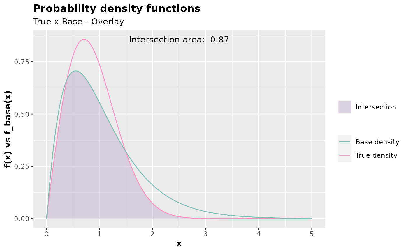
# Considering c = 1 (default)
inspect(
   f = dweibull,
   f_base = dgamma,
   xlim = c(0,5),
   args_f = list(shape = 2, scale = 1),
   args_f_base = list(shape = 2.1, rate = 2),
   c = 1
)


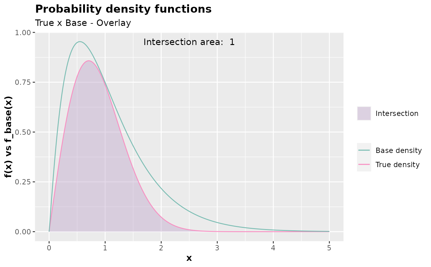
# Considering c = 1.35.
inspect(
   f = dweibull,
   f_base = dgamma,
   xlim = c(0,5),
   args_f = list(shape = 2, scale = 1),
   args_f_base = list(shape = 2.1, rate = 2),
   c = 1.35
)


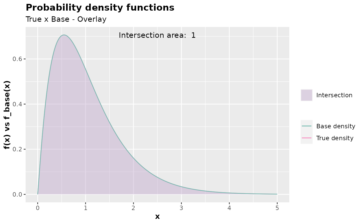
# Plotting f equal to f_base. This would be the best-case scenario, which,
# in practice, is unlikely.
inspect(
   f = dgamma,
   f_base = dgamma,
   xlim = c(0,5),
   args_f = list(shape = 2.1, rate = 2),
   args_f_base = list(shape = 2.1, rate = 2),
   c = 1
)