Specifying a base probability density function

Motivation

Providing a more suitable probability density function can further reduce computational cost and increase the acceptance probability. Therefore, inspecting an alternative for the base probability density function is a good practice.

The accept_reject() function supports, for the continuous case, specifying a base probability density function if you don’t want to use the continuous uniform distribution as the default base.

When choosing to specify another probability density function different from the uniform one, it’s necessary to specify the following arguments:

• f_base: base probability density function;
• random_base: sampling from the base probability density function;
• args_f_base: list with the parameters of the base density.

By default, all of them are NULL, and the continuous uniform distribution in xlim is used as the base. If at least one of these arguments is not specified, no error will occur, and the continuous uniform distribution in xlim will still be used as the base.

For the discrete case, if the user mistakenly specifies any of these arguments, i.e., when continuous = FALSE, the accept_reject() function will ignore these arguments and use the discrete uniform distribution as the base.

If you choose to specify a base density, it’s convenient to inspect it by comparing the base density function with the theoretical probability density function. The inspect() function facilitates this task. The inspect() function will plot the base probability density function and the theoretical probability density function, find the intersection between the densities, and display the value of the intersection area on the plot. These are important pieces of information to decide if the base probability density function specified in the args_f_base argument and the value of c (default is 1) are appropriate.

Example of inspection

library(AcceptReject)
#> 
#> Attaching package: 'AcceptReject'
#> The following object is masked from 'package:stats':
#> 
#>     qqplot

library(cowplot) # install.packages("cowplot")

# Ensuring reproducibility
set.seed(0)

# Inspecting
# Case a
a <- inspect(
  f = dweibull,
  args_f = list(shape = 2.1, scale = 2.2),
  f_base = dgamma,
  args_f_base = list(shape = 2.8, rate = 1.2),
  xlim = c(0, 10),
  c = 1.2
)

# Inspecting
# Case b
b <- inspect(
  f = dweibull,
  args_f = list(shape = 2.1, scale = 2.2),
  f_base = dgamma,
  args_f_base = list(shape = 2.9, rate = 2.5),
  xlim = c(0, 10),
  c = 1.4
)

plot_grid(a, b, nrow = 2L, labels = c("a", "b"))

Notice that considering the distribution in scenario “a” in the code above is more convenient. Note that the area is approximately 1, the base probability density function with parameters shape = 2.8 and rate = 1.2 provides a shape close to the theoretical distribution, and c = 1.2 ensures that the base density function upper bounds the theoretical probability density function. Therefore, considering f_base with \(\Gamma(\alpha = 2.8, \beta = 1.2)\) and c = 1.2 is a reasonable choice for a base distribution.

Therefore, passing arguments to f_base = dgamma, args_f_base = list(shape = 2.8, rate = 1.2), and c = 1.2 to the accept_reject() function will lead us to an even more efficient code.

library(AcceptReject)
library(tictoc) # install.packages("tictoc")

# Ensuring reproducibility
set.seed(0)

# Não especificando a função densidade de probabilidade base

tic()
case_1 <- accept_reject(
  n = 200e3L,
  continuous = TRUE,
  f = dweibull,
  args_f = list(shape = 2.1, scale = 2.2),
  xlim = c(0, 10)
)
toc()
#> 0.076 sec elapsed

# Specifying the base probability density function
tic()
case_2 <- accept_reject(
  n = 200e3L,
  continuous = TRUE,
  f = dweibull,
  args_f = list(shape = 2.1, scale = 2.2),
  f_base = dgamma,
  random_base = rgamma,
  args_f_base = list(shape = 2.8, rate = 1.2),
  xlim = c(0, 10),
  c = 1.2
)
toc()
#> 0.082 sec elapsed

# Visualizing the results
p1 <- plot(case_1)
p2 <- plot(case_2)

plot_grid(p1, p2, nrow = 2L)

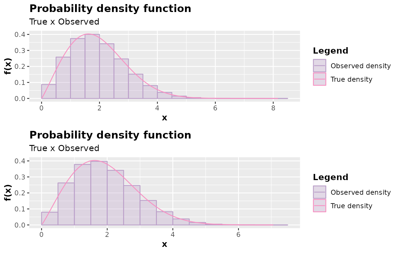
Notice that the results were very close in a graphical analysis. However, the execution time specifying a convenient base density was lower for a very large sample.

Important:

You can investigate and try inspecting a base probability density function to find a specification of the base density and a value of c that you can pass as an argument to accept_reject(). The idea is to find a small value of c to maximize the acceptance probability and pass this value to stat_c so that the accept_reject() function can improve this value.