Acceptance-Rejection Method

This function implements the acceptance-rejection method for generating random numbers from a given probability density function (pdf).

Usage

accept_reject(
  n = 1L,
  continuous = TRUE,
  f = NULL,
  args_f = NULL,
  f_base = NULL,
  random_base = NULL,
  args_f_base = NULL,
  xlim = NULL,
  c = NULL,
  parallel = FALSE,
  cores = NULL,
  warning = TRUE,
  ...
)

Arguments

n: The number of random numbers to generate.
continuous: A logical value indicating whether the pdf is continuous or discrete. Default is TRUE.
f: The probability density function (continuous = TRUE), in the continuous case or the probability mass function, in the discrete case (continuous = FALSE).
args_f: A list of arguments to be passed to the f function. It refers to the list of arguments of the target distribution.
f_base: Base probability density function (for continuous case).If f_base = NULL, a uniform distribution will be used. In the discrete case, this argument is ignored, and a uniform probability mass function will be used as the base.
random_base: Random number generation function for the base distribution passed as an argument to f_base. If random_base = NULL (default), the uniform generator will be used. In the discrete case, this argument is disregarded, and the uniform random number generator function will be used.
args_f_base: A list of arguments for the base distribution. This refers to the list of arguments that will be passed to the function f_base. It will be disregarded in the discrete case.
xlim: A vector specifying the range of values for the random numbers in the form c(min, max). Default is c(0, 100).
c: A constant value used in the acceptance-rejection method. If NULL, c will be estimated automatically.
parallel: A logical value indicating whether to use parallel processing for generating random numbers. Default is FALSE.
cores: The number of cores to be used in parallel processing. Default is NULL, i.e, all available cores.
warning: A logical value indicating whether to show warnings. Default is TRUE.
...: Additional arguments to be passed to the optimize(). With this argument, it is possible to change the tol argument of optimize(). Default is tol = .Machine$double.eps^0.25).

Value

A vector of random numbers generated using the acceptance-rejection method. The return is an object of class accept_reject, but it can be treated as an atomic vector.

Details

In situations where we cannot use the inversion method (situations where it is not possible to obtain the quantile function) and we do not know a transformation that involves a random variable from which we can generate observations, we can use the acceptance and rejection method. Suppose that $X$ and $Y$ are random variables with probability density function (pdf) or probability function (pf) $f$ and $g$, respectively. In addition, suppose that there is a constant $c$ such that

$$f(x) \leq c \cdot g(x), \quad \forall x \in \mathbb{R}.$$

for all values of $t$, with $f(t)>0$. To use the acceptance and rejection method to generate observations from the random variable $X$, using the algorithm below, first find a random variable $Y$ with pdf or pf $g$, that satisfies the above condition.

Algorithm of the Acceptance and Rejection Method:

1 - Generate an observation $y$ from a random variable $Y$ with pdf/pf $g$;

2 - Generate an observation $u$ from a random variable $U\sim \mathcal{U} (0, 1)$;

3 - If $u < \frac{f(y)}{cg(y)}$ accept $x = y$; otherwise reject $y$ as an observation of the random variable $X$ and return to step 1.

Proof: Let's consider the discrete case, that is, $X$ and $Y$ are random variables with pf's $f$ and $g$, respectively. By step 3 of the above algorithm, we have that ${accept} = {x = y} = u < \frac{f(y)}{cg(y)}$. That is,

$P(accept | Y = y) = \frac{P(accept \cap {Y = y})}{g(y)} = \frac{P(U \leq f(y)/cg(y)) \times g(y)}{g(y)} = \frac{f(y)}{cg(y)}.$

Hence, by the Total Probability Theorem, we have that:

$P(accept) = \sum_y P(accept|Y=y)\times P(Y=y) = \sum_y \frac{f(y)}{cg(y)}\times g(y) = \frac{1}{c}.$

Therefore, by the acceptance and rejection method we accept the occurrence of $Y$ as being an occurrence of $X$ with probability $1/c$. In addition, by Bayes' Theorem, we have that

$P(Y = y | accept) = \frac{P(accept|Y = y)\times g(y)}{P(accept)} = \frac{[f(y)/cg(y)] \times g(y)}{1/c} = f(y).$

The result above shows that accepting $x = y$ by the procedure of the algorithm is equivalent to accepting a value from $X$ that has pf $f$.

The argument c = NULL is the default. Thus, the function accept_reject() estimates the value of c using the optimization algorithm optimize() using the Brent method. For more details, see optimize() function. If a value of c is provided, the function accept_reject() will use this value to generate the random observations. An inappropriate choice of c can lead to low efficiency of the acceptance and rejection method.

In Unix-based operating systems, the function accept_reject() can be executed in parallel. To do this, simply set the argument parallel = TRUE. The function accept_reject() utilizes the parallel::mclapply() function to execute the acceptance and rejection method in parallel. On Windows operating systems, the code will not be parallelized even if parallel = TRUE is set.

For the continuous case, a base density function can be used, where the arguments f_base, random_base and args_f_base need to be passed. If at least one of them is NULL, the function will assume a uniform density function over the interval xlim.

For the discrete case, the arguments f_base, random_base and args_f_base should be NULL, and if they are passed, they will be disregarded, as for the discrete case, the discrete uniform distribution will always be considered as the base. Sampling from the discrete uniform distribution has shown good performance for the discrete case.

The advantage of using parallelism in Unix-based systems is relative and should be tested for each case. Significant improvement is observed when considering parallelism for very large values of n. It is advisable to conduct benchmarking studies to evaluate the efficiency of parallelism in a practical situation.

References

BISHOP, Christopher. 11.4: Slice sampling. Pattern Recognition and Machine Learning. Springer, 2006.

Brent, R. (1973) Algorithms for Minimization without Derivatives. Englewood Cliffs N.J.: Prentice-Hall.

CASELLA, George; ROBERT, Christian P.; WELLS, Martin T. Generalized accept-reject sampling schemes. Lecture Notes-Monograph Series, p. 342-347, 2004.

NEUMANN V (1951). “Various techniques used in connection with random digits.” Notes by GE Forsythe, pp. 36–38.

NEAL, Radford M. Slice sampling. The Annals of Statistics, v. 31, n. 3, p. 705-767, 2003.

Examples

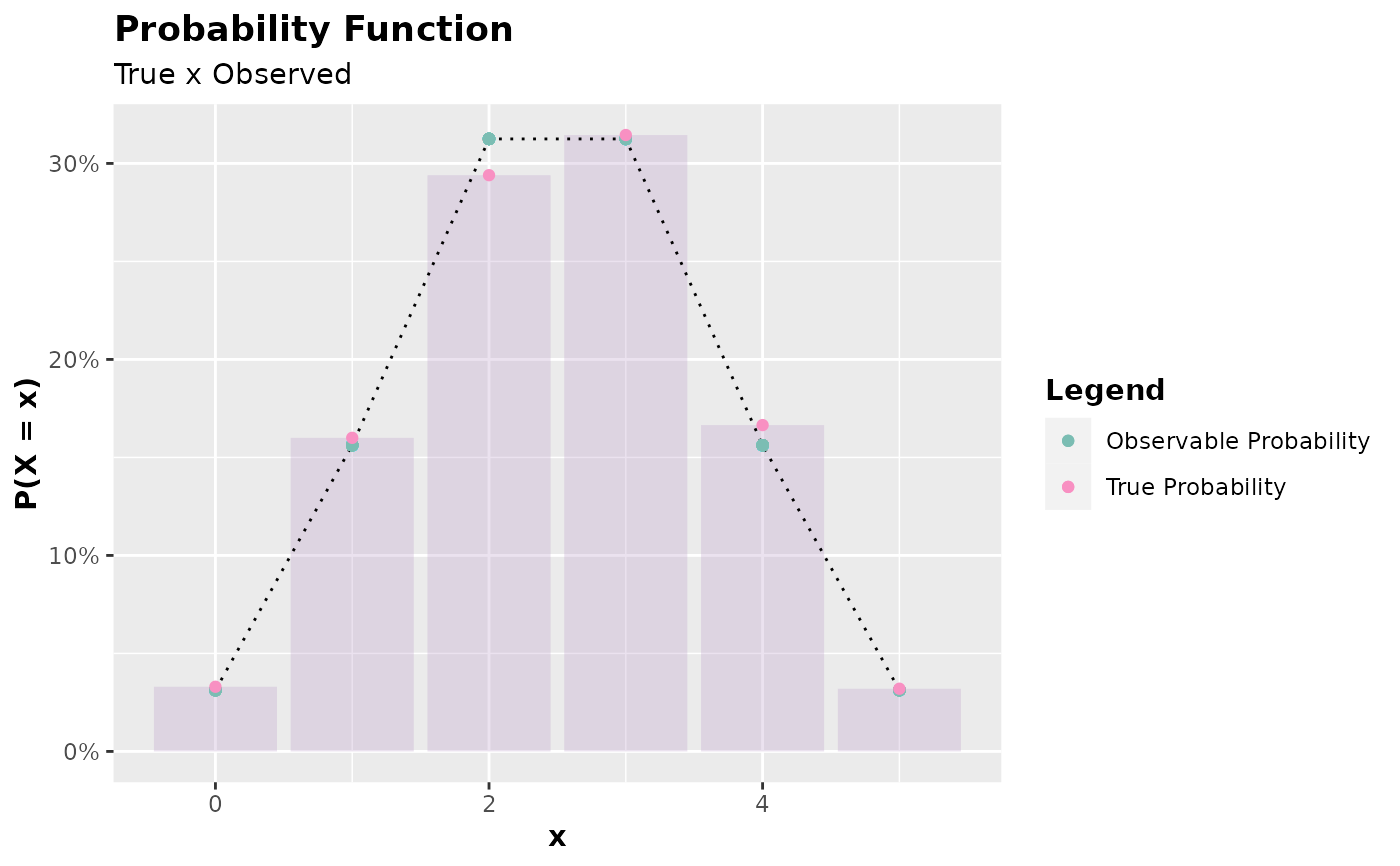
set.seed(0) # setting a seed for reproducibility

x <- accept_reject(
  n = 2000L,
  f = dbinom,
  continuous = FALSE,
  args_f = list(size = 5, prob = 0.5),
  xlim = c(0, 5)
)
#> ! Warning: f(5) is 0.03125. If f is defined for x >= 5, trying a upper limit might be better.
plot(x)


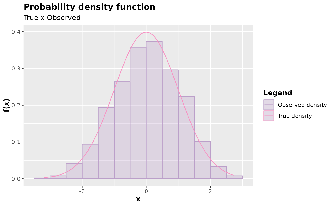
y <- accept_reject(
  n = 1000L,
  f = dnorm,
  continuous = TRUE,
  args_f = list(mean = 0, sd = 1),
  xlim = c(-4, 4)
)
plot(y)