QQ-Plot Plot the QQ-Plot between observed quantiles and theoretical quantiles.

Usage

# S3 method for accept_reject
qqplot(
  x,
  alpha = 0.5,
  color_points = "#F890C2",
  color_line = "#BB9FC9",
  size_points = 1,
  size_line = 1,
  ...
)

Arguments

x: Object of the class accept_reject returned by the function accept_reject().
alpha: Transparency of the points and reference line representing where the quantiles should be (theoretical quantiles).
color_points: Color of the points (default is "#F890C2").
color_line: Color of the reference line (detault is "#BB9FC9").
size_points: Size of the points (default is 1).
size_line: Thickness of the reference line (default is 1).
...: Additional arguments for the quantile() function. For instance, it's possible to change the algorithm type for quantile calculation.

Value

An object of classes gg and ggplot with the QQ-Plot between the observed quantiles generated by the return of the function accept_reject()

and the theoretical quantiles of the true distribution.

Details

The function qqplot.accept_reject() for samples larger than ten thousand, the geom_scattermost() function from the scattermore library is used to plot the points, as it is more efficient than geom_point() from the ggplot2 library.

Examples

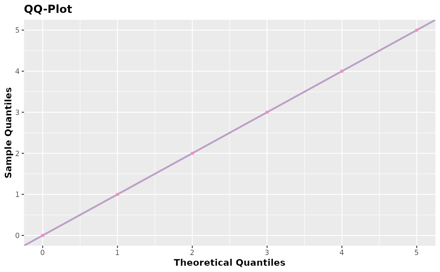
set.seed(0) # setting a seed for reproducibility

x <- accept_reject(
  n = 2000L,
  f = dbinom,
  continuous = FALSE,
  args_f = list(size = 5, prob = 0.5),
  xlim = c(0, 5)
)
#> ! Warning: f(5) is 0.03125. If f is defined for x >= 5, trying a upper limit might be better.
qqplot(x)


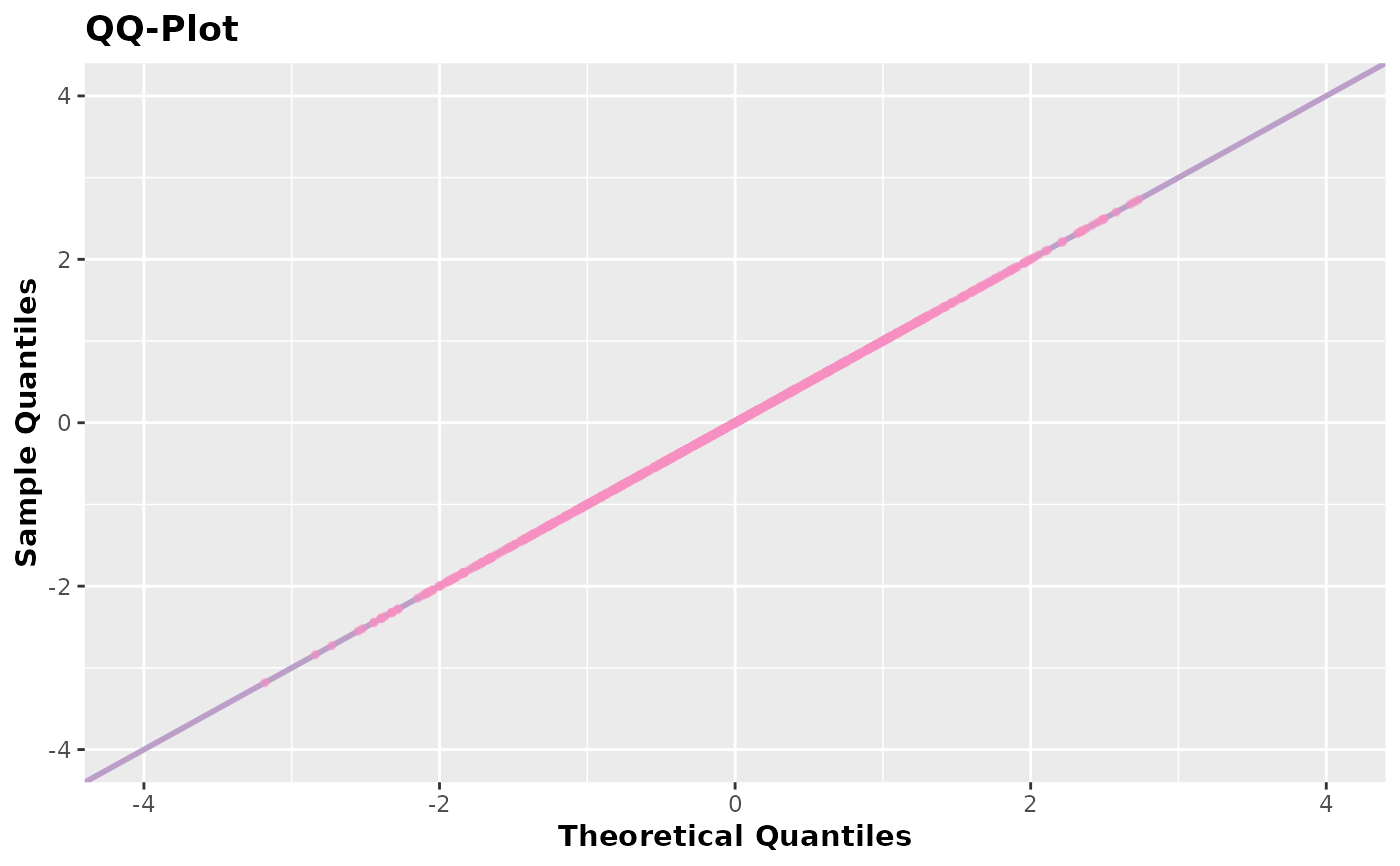
y <- accept_reject(
  n = 1000L,
  f = dnorm,
  continuous = TRUE,
  args_f = list(mean = 0, sd = 1),
  xlim = c(-4, 4)
)
qqplot(y)