Heteroskedasticity-consistent covariance estimator

Computes a heteroskedasticity-consistent covariance matrix estimator for an ordinary least squares model fitted with stats::lm(). The function returns a rich S3 object that stores the covariance matrix, HC weights, leverage values, method parameters, and model metadata.

Usage

vcov_hc(object, type = "hcbeta", ...)

Arguments

object: An ordinary least squares model fitted by stats::lm().
type: A character string specifying the HC estimator. The default is "hcbeta".
...: Method-specific constants. Unknown names are rejected. See Details for the accepted names, defaults, and parameter domains.

Value

An object of class hcinfer_vcov. The covariance matrix is stored in object$vcov and is returned directly by vcov().

Details

For a linear model with design matrix $X$, OLS residuals $\hat e_t$, and HC weights $g_t$, the estimator is

$$\widehat{\Psi}_{HC} = (X'X)^{-1} X' \widehat{\Omega} X (X'X)^{-1},$$

where $\widehat{\Omega} = diag(\hat e_t^2 g_t)$. The supported estimators are "hc0", "hc1", "hc2", "hc3", "hc4", "hc4m", "hc5", "hc5m", and "hcbeta".

Additional arguments in ... are method-specific. The defaults are:

"hc0", "hc1", "hc2", "hc3", "hc4", and "hc4m": no method-specific arguments.
"hc5": k = 0.7.
"hc5m": k = 0.7, k1 = 1, k2 = 0, k3 = 1, gamma1 = 1, and gamma2 = 1.5.
"hcbeta": c1 = 7, c2 = 0.75, lower = 0.01, and upper = 0.99.

For "hc5" and "hc5m", k, k1, k2, and k3 must be nonnegative, while gamma1 and gamma2 must be positive. For "hcbeta", c1 must be nonnegative, c2 must be positive, and lower and upper must lie in (0, 1) with lower < upper. The HCbeta truncation is $w_t = max(lower, min(1 - h_t, upper))$.

References

White, H. (1980). A heteroskedasticity-consistent covariance matrix estimator and a direct test for heteroskedasticity. Econometrica, 48(4), 817-838. doi:10.2307/1912934

Hinkley, D. V. (1977). Jackknifing in unbalanced situations. Technometrics, 19(3), 285-292. doi:10.1080/00401706.1977.10489550

Horn, S. D., Horn, R. A., and Duncan, D. B. (1975). Estimating heteroscedastic variances in linear models. Journal of the American Statistical Association, 70(350), 380-385. doi:10.1080/01621459.1975.10479877

MacKinnon, J. G. and White, H. (1985). Some heteroskedasticity-consistent covariance matrix estimators with improved finite sample properties. Journal of Econometrics, 29(3), 305-325. doi:10.1016/0304-4076(85)90158-7

Davidson, R. and MacKinnon, J. G. (1993). Estimation and Inference in Econometrics. Oxford University Press.

Cribari-Neto, F. (2004). Asymptotic inference under heteroskedasticity of unknown form. Computational Statistics and Data Analysis, 45(2), 215-233. doi:10.1016/S0167-9473(02)00366-3

Cribari-Neto, F. and da Silva, W. B. (2011). A new heteroskedasticity consistent covariance matrix estimator for the linear regression model. AStA Advances in Statistical Analysis, 95(2), 129-146. doi:10.1007/s10182-010-0141-2

Cribari-Neto, F., Souza, T. C., and Vasconcellos, K. L. P. (2007). Inference under heteroskedasticity and leveraged data. Communications in Statistics - Theory and Methods, 36(10), 1877-1888. doi:10.1080/03610920601126589

Li, S., Zhang, N., Zhang, X., and Wang, G. (2016). A new heteroskedasticity-consistent covariance matrix estimator and inference under heteroskedasticity. Journal of Statistical Computation and Simulation, 87(1), 198-210. doi:10.1080/00949655.2016.1198906

Examples

schools <- PublicSchools |>
  dplyr::mutate(
    income_scaled = income / 10000,
    income_scaled_sq = income_scaled^2
  )
fit <- lm(expenditure ~ income_scaled + income_scaled_sq, data = schools)
cov <- vcov_hc(fit, type = "hcbeta")
cov
#> 
#> ── 🥪 HCbeta robust covariance ─────────────────────────────────────────────────
#> 📐 Model: `expenditure ~ income_scaled + income_scaled_sq`
#> Dimension: 3 x 3
#> Observations: 50
#> Parameters: 3
#> 🎯 Maximum leverage: 0.6508
#> ⚖️ Maximum robust weight: 4.5807
#> Use `vcov()` to extract the stored covariance matrix.
vcov(cov)
#>                  (Intercept) income_scaled income_scaled_sq
#> (Intercept)         723617.6      -1962262          1312195
#> income_scaled     -1962262.2       5329884         -3569755
#> income_scaled_sq   1312195.3      -3569755          2394627
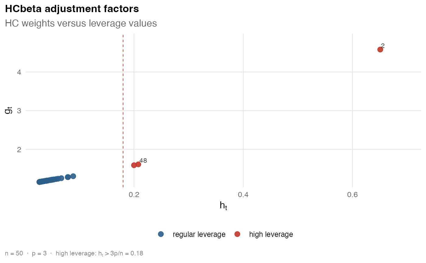
plot(cov)


vcov_hc(fit, type = "hcbeta", c1 = 7, c2 = 0.75, lower = 0.01, upper = 0.99)
#> 
#> ── 🥪 HCbeta robust covariance ─────────────────────────────────────────────────
#> 📐 Model: `expenditure ~ income_scaled + income_scaled_sq`
#> Dimension: 3 x 3
#> Observations: 50
#> Parameters: 3
#> 🎯 Maximum leverage: 0.6508
#> ⚖️ Maximum robust weight: 4.5807
#> Use `vcov()` to extract the stored covariance matrix.
vcov_hc(fit, type = "hc5", k = 0.7)
#> 
#> ── 🥪 HC5 robust covariance ────────────────────────────────────────────────────
#> 📐 Model: `expenditure ~ income_scaled + income_scaled_sq`
#> Dimension: 3 x 3
#> Observations: 50
#> Parameters: 3
#> 🎯 Maximum leverage: 0.6508
#> ⚖️ Maximum robust weight: 2946.7866
#> Use `vcov()` to extract the stored covariance matrix.
vcov_hc(fit, type = "hc5m", k = 0.7, k1 = 1, k2 = 0, k3 = 1)
#> 
#> ── 🥪 HC5m robust covariance ───────────────────────────────────────────────────
#> 📐 Model: `expenditure ~ income_scaled + income_scaled_sq`
#> Dimension: 3 x 3
#> Observations: 50
#> Parameters: 3
#> 🎯 Maximum leverage: 0.6508
#> ⚖️ Maximum robust weight: 8438.7828
#> Use `vcov()` to extract the stored covariance matrix.