Pairs bootstrap inference with hcinfer • hcinfer

The pairs (case) bootstrap is a resampling method for the coefficients of an ordinary least squares model. It resamples whole observations, refits the model many times, and summarizes the resulting spread of the estimates. Because it makes no assumption about the form of the error variance, it is a natural empirical companion to the analytic heteroskedasticity-consistent (HC) standard errors that hcinfer computes, and this vignette shows how to run it, read its output, and compare it with the HC estimators.

The method

For each replicate the bootstrap draws n rows with replacement from the original data and refits OLS on that resample. Writing the estimate on replicate r as the vector of refitted coefficients, the bootstrap standard error of a coefficient is the standard deviation of its replicate values. boot_pairs() offers three interval types: "percentile" uses the empirical quantiles of the replicates, "basic" (reverse percentile) reflects those quantiles about the original estimate, and "normal" uses the estimate plus or minus a normal quantile times the bootstrap standard error.

Data and model

library(hcinfer)

schools <- PublicSchools
schools$income_scaled <- schools$income / 10000
schools$income_scaled_sq <- schools$income_scaled^2

fit <- lm(expenditure ~ income_scaled + income_scaled_sq, data = schools)
fit
#> 
#> Call:
#> lm(formula = expenditure ~ income_scaled + income_scaled_sq, 
#>     data = schools)
#> 
#> Coefficients:
#>      (Intercept)     income_scaled  income_scaled_sq  
#>            832.9           -1834.2            1587.0

Running the bootstrap

A single call fits the resamples and stores the estimates, standard errors, bias, and intervals. Supplying seed makes the run reproducible.

boot <- boot_pairs(fit, B = 2000, seed = 123)
boot
#> 
#> ── Pairs bootstrap inference ───────────────────────────────────────────────────
#> Model: `expenditure ~ income_scaled + income_scaled_sq`
#> Observations: 50 | Parameters: 3
#> Replicates: 2000 of 2000 valid | Interval: percentile at 95.0%
#> Execution: sequential | Seed: 123
#> # A tibble: 3 × 5
#>   term             estimate bias   boot_se ci            
#>   <chr>            <chr>    <chr>  <chr>   <chr>         
#> 1 (Intercept)      832.9    -238.7 637.4   [-649.6, 1492]
#> 2 income_scaled    -1834    648    1722    [-3501, 2165] 
#> 3 income_scaled_sq 1587     -433   1151    [-1085, 2626]

Extractors

The coef(), vcov(), and confint() methods pull out the pieces you need. coef() returns the original OLS estimates, vcov() the bootstrap covariance matrix, and confint() the interval table.

coef(boot)
#>      (Intercept)    income_scaled income_scaled_sq 
#>         832.9144       -1834.2029        1587.0423
vcov(boot)
#>                  (Intercept) income_scaled income_scaled_sq
#> (Intercept)         406215.5      -1096583           730159
#> income_scaled     -1096582.6       2966936         -1979795
#> income_scaled_sq    730159.0      -1979795          1323952
confint(boot)
#> # A tibble: 3 × 4
#>   term             conf_low conf_high level
#>   <chr>               <dbl>     <dbl> <dbl>
#> 1 (Intercept)         -650.     1492.  0.95
#> 2 income_scaled      -3501.     2165.  0.95
#> 3 income_scaled_sq   -1085.     2626.  0.95

confint() can recompute intervals at a different level or type directly from the stored replicates, without rerunning the bootstrap.

confint(boot, level = 0.99, type = "basic")
#> # A tibble: 3 × 4
#>   term             conf_low conf_high level
#>   <chr>               <dbl>     <dbl> <dbl>
#> 1 (Intercept)         -14.8     2511.  0.99
#> 2 income_scaled     -6417.       327.  0.99
#> 3 income_scaled_sq    176.      4624.  0.99
confint(boot, parm = "income_scaled_sq", level = 0.90)
#> # A tibble: 1 × 4
#>   term             conf_low conf_high level
#>   <chr>               <dbl>     <dbl> <dbl>
#> 1 income_scaled_sq    -902.     2524.   0.9

Visualizing the intervals

plot() draws each coefficient as its estimate with its bootstrap interval, colored by whether the interval excludes zero.

plot(boot)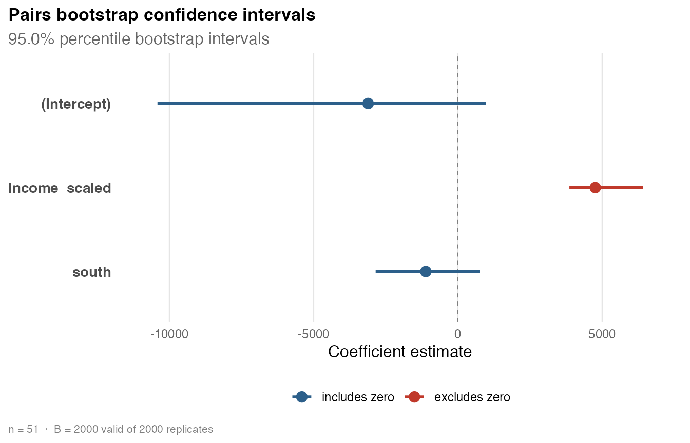

Pairs bootstrap confidence intervals for the public-schools regression coefficients.

An empirical reference for HC standard errors

Because the pairs bootstrap assumes nothing about the error variance, its standard errors are a useful cross-check on the analytic HC estimators. The following table places the OLS, bootstrap, HCbeta, and HC3 standard errors side by side.

data.frame(
  term = boot$table$term,
  ols = sqrt(diag(vcov(fit))),
  bootstrap = boot$table$std_error,
  hcbeta = sqrt(diag(vcov(hcinfer(fit, type = "hcbeta")))),
  hc3 = sqrt(diag(vcov(hcinfer(fit, type = "hc3"))))
)
#>                              term      ols bootstrap    hcbeta      hc3
#> (Intercept)           (Intercept) 327.2925  637.3504  850.6572 1095.001
#> income_scaled       income_scaled 828.9855 1722.4796 2308.6541 2975.411
#> income_scaled_sq income_scaled_sq 519.0768 1150.6312 1547.4583 1995.242

The bootstrap and HC standard errors should tell a similar story; large disagreements are worth investigating, often through high-leverage points.

Reproducibility

With a fixed seed, two runs are identical, and the call restores the caller’s random-number stream so it does not disturb a surrounding analysis.

a <- boot_pairs(fit, B = 1000, seed = 7)
b <- boot_pairs(fit, B = 1000, seed = 7)
identical(a$replicates, b$replicates)
#> [1] TRUE

Running in parallel

For large B or large n, set cores to 2 or more to distribute the replicate fits across worker processes (requires the mirai and carrier packages). The numeric result is identical to a sequential run with the same seed; parallelism only changes the speed. The default cores = 1 runs sequentially.

boot_pairs(fit, B = 10000, cores = 4, seed = 1)

Practical guidance

Use a few thousand replicates for stable standard errors and more for stable tail quantiles of the percentile and basic intervals. Choose ci_type to match your needs: percentile and basic intervals adapt to skewness in the replicate distribution, while normal intervals are symmetric. If a resample is rank deficient it is dropped with a warning, and the summaries use the remaining replicates.