hcinfer

hcinfer computes heteroskedasticity-consistent covariance estimators and normal Wald inference for ordinary least squares models. The currently implemented covariance matrix estimators are listed below.

Implemented Estimators

The table below is generated by hc_methods() and lists the covariance matrix estimators currently implemented in hcinfer.

type	label	description	default_arguments
hc0	HC0	White heteroskedasticity-consistent estimator.	none
hc1	HC1	HC0 with degrees-of-freedom scaling.	none
hc2	HC2	Leverage-adjusted estimator with exponent 1.	none
hc3	HC3	Leverage-adjusted estimator with exponent 2.	none
hc4	HC4	Adaptive leverage correction by Cribari-Neto.	none
hc4m	HC4m	Modified HC4 correction by Cribari-Neto and da Silva.	none
hc5	HC5	High-leverage correction by Cribari-Neto, Souza, and Vasconcellos.	k = 0.7
hc5m	HC5m	Modified HC5 correction by Li, Zhang, Zhang, and Wang.	k = 0.7, k1 = 1, k2 = 0, k3 = 1, gamma1 = 1, gamma2 = 1.5
hcbeta	HCbeta	Beta-distribution leverage correction.	c1 = 7, c2 = 0.75, lower = 0.01, upper = 0.99

Installation

# install.packages("hcinfer")

# Development version
remotes::install_github("prdm0/hcinfer")

Basic Use

library(hcinfer)

schools <- PublicSchools
schools$income_scaled <- schools$income / 10000
schools$income_scaled_sq <- schools$income_scaled^2

fit <- lm(expenditure ~ income_scaled + income_scaled_sq, data = schools)

result <- hcinfer(fit)

The default estimator is HCbeta. Use tests() and confint() to extract the main inferential quantities as tibbles.

tests(result)
#> # A tibble: 3 × 8
#>   term             estimate null_value std_error z_value p_value alpha reject
#>   <chr>               <dbl>      <dbl>     <dbl>   <dbl>   <dbl> <dbl> <lgl> 
#> 1 (Intercept)          833.          0      851.   0.979   0.328  0.05 FALSE 
#> 2 income_scaled      -1834.          0     2309.  -0.794   0.427  0.05 FALSE 
#> 3 income_scaled_sq    1587.          0     1547.   1.03    0.305  0.05 FALSE
confint(result)
#> # A tibble: 3 × 4
#>   term             conf_low conf_high level
#>   <chr>               <dbl>     <dbl> <dbl>
#> 1 (Intercept)         -834.     2500.  0.95
#> 2 income_scaled      -6359.     2691.  0.95
#> 3 income_scaled_sq   -1446.     4620.  0.95

Confidence Intervals

The plot() method displays the robust confidence intervals and marks the null value used in the tests.

plot(result)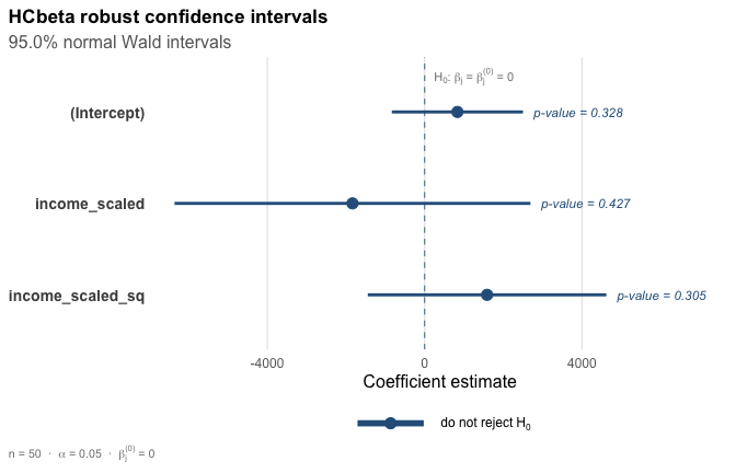

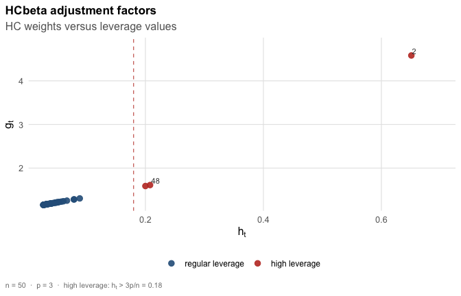
Diagnostics

Use vcov_hc() when you only need the robust covariance matrix and its diagnostics. The plot() method for this object shows leverage values and HC adjustment factors.

cov_hcbeta <- vcov_hc(fit)
plot(cov_hcbeta)

Main Functions

hc_methods()
coef(result)
vcov(result)

The most common workflow is:

fit <- lm(y ~ x1 + x2, data = data)
result <- hcinfer(fit, type = "hcbeta")

summary(result)
tests(result)
confint(result)
plot(result)

Learn More

Start with vignette("introduction", package = "hcinfer") for a compact overview of the package API.

References

• White, H. (1980). A heteroskedasticity-consistent covariance matrix estimator and a direct test for heteroskedasticity. Econometrica, 48(4), 817-838.
• Cribari-Neto, F. (2004). Asymptotic inference under heteroskedasticity of unknown form. Computational Statistics and Data Analysis, 45(2), 215-233.
• Cribari-Neto, F., Cunha, M. O., and Marinho, P. R. D. (2025). HCbeta: A beta-distribution-based heteroskedasticity-consistent covariance estimator. Working paper.