This vignette gives a compact overview of hcinfer. It
uses only base R for data preparation, then shows the main functions,
extraction methods, and plots.
Data and Model
The examples use the PublicSchools data included with
the package. The model is the quadratic income model used in the HCbeta
application.
library(hcinfer)

schools <- PublicSchools
schools$income_scaled <- schools$income / 10000
schools$income_scaled_sq <- schools$income_scaled^2

fit <- lm(expenditure ~ income_scaled + income_scaled_sq, data = schools)
fit
#>
#> Call:
#> lm(formula = expenditure ~ income_scaled + income_scaled_sq,
#>     data = schools)
#>
#> Coefficients:
#>      (Intercept)     income_scaled  income_scaled_sq
#>            832.9           -1834.2            1587.0
The call to lm() omits observations with missing model
variables.
Available Estimators
Use hc_methods() to list the estimators and their
default arguments.
hc_methods()
#> # A tibble: 9 × 4
#>   type   label  description                                    default_arguments
#>   <chr>  <chr>  <chr>                                          <chr>
#> 1 hc0    HC0    White heteroskedasticity-consistent estimator. none
#> 2 hc1    HC1    HC0 with degrees-of-freedom scaling.           none
#> 3 hc2    HC2    Leverage-adjusted estimator with exponent 1.   none
#> 4 hc3    HC3    Leverage-adjusted estimator with exponent 2.   none
#> 5 hc4    HC4    Adaptive leverage correction by Cribari-Neto.  none
#> 6 hc4m   HC4m   Modified HC4 correction by Cribari-Neto and d… none
#> 7 hc5    HC5    High-leverage correction by Cribari-Neto, Sou… k = 0.7
#> 8 hc5m   HC5m   Modified HC5 correction by Li, Zhang, Zhang, … k = 0.7, k1 = 1,…
#> 9 hcbeta HCbeta Beta-distribution leverage correction.         c1 = 7, c2 = 0.7…
The available types are "hc0", "hc1",
"hc2", "hc3", "hc4",
"hc4m", "hc5", "hc5m", and
"hcbeta".
Robust Inference
Use hcinfer() to perform heteroskedasticity-robust
inference for an lm() object. The default estimator is
HCbeta.
result <- hcinfer(fit)
result
#>
#> ── HCbeta robust inference ─────────────────────────────────────────────────────
#> Model: `expenditure ~ income_scaled + income_scaled_sq`
#> Observations: 50 | Parameters: 3
#> Robust covariance: HCbeta
#> Confidence level: 95.0% | Normal critical value: 1.9600
#> Use `summary()` for p-values, test results, confidence intervals, and
#> diagnostics.
Use summary() for a readable report with tests on
regression coefficients, confidence intervals, leverage diagnostics, and
heteroskedasticity-robust diagnostics.
summary(result)
#>
#> ── HCbeta robust inference summary ─────────────────────────────────────────────
#>
#> ── Model ──
#>
#> Formula: `expenditure ~ income_scaled + income_scaled_sq`
#> Observations: 50 | Parameters: 3 | Residual df: 47
#>
#> ── Robust covariance ──
#>
#> Estimator: HCbeta
#> Confidence level: 95.0% | Normal critical value: 1.9600
#> Tests are two-sided normal Wald tests, one coefficient at a time.
#> Test results use alpha = 0.050.
#>
#> ── Leverage diagnostics ──
#>
#> # A tibble: 6 × 2
#>   statistic value
#>   <chr>     <chr>
#> 1 minimum   0.02669
#> 2 q1        0.03106
#> 3 median    0.03912
#> 4 mean      0.06
#> 5 q3        0.04962
#> 6 maximum   0.6508
#> Maximum leverage: observation 2 (index 2), value 0.6508
#> Average leverage: 0.0600
#> Concentration: 10.85 x average leverage
#>
#> ── Robust weights ──
#>
#> # A tibble: 6 × 2
#>   statistic value
#>   <chr>     <chr>
#> 1 minimum   1.156
#> 2 q1        1.167
#> 3 median    1.187
#> 4 mean      1.276
#> 5 q3        1.212
#> 6 maximum   4.581
#> Maximum weight: observation 2 (index 2), value 4.5807
#> Median weight: 1.1869
#> Concentration: 3.86 x median weight
#>
#> ── Method parameters ──
#>
#> # A tibble: 12 × 3
#>    parameter value    role
#>    <chr>     <chr>    <chr>
#>  1 c1        7        method constant
#>  2 c2        0.75     method constant
#>  3 lower     0.01     method constant
#>  4 upper     0.99     method constant
#>  5 mu_hat    0.94     estimated quantity
#>  6 s2_w      0.008504 estimated quantity
#>  7 phi_hat   5.632    estimated quantity
#>  8 a_hat     5.294    estimated quantity
#>  9 b_hat     0.3379   estimated quantity
#> 10 zeta      0.5      estimated quantity
#> 11 a_tilde   3.147    estimated quantity
#> 12 b_tilde   0.669    estimated quantity
#>
#> ── Coefficient tests ──
#>
#> # A tibble: 3 × 9
#>   term             estimate robust_se z       p_value alpha test_result
#>   <chr>            <chr>    <chr>     <chr>   <chr>   <chr> <chr>
#> 1 (Intercept)      832.9    850.7     0.9791  0.328   0.050 do not reject H0
#> 2 income_scaled    -1834    2309      -0.7945 0.427   0.050 do not reject H0
#> 3 income_scaled_sq 1587     1547      1.026   0.305   0.050 do not reject H0
#>   ci             ci_relation
#>   <chr>          <chr>
#> 1 [-834.3, 2500] includes null
#> 2 [-6359, 2691]  includes null
#> 3 [-1446, 4620]  includes null
#>
#> ── Confidence intervals ──
#>
#> # A tibble: 3 × 4
#>   term             null_value interval       interpretation
#>   <chr>            <chr>      <chr>          <chr>
#> 1 (Intercept)      0          [-834.3, 2500] includes null
#> 2 income_scaled    0          [-6359, 2691]  includes null
#> 3 income_scaled_sq 0          [-1446, 4620]  includes null
#> test_result is based on p_value < alpha. Do not reject H0 does not mean that H0
#> is true.
You can choose another covariance matrix estimator with
type.
result_hc3 <- hcinfer(fit, type = "hc3")
result_hc3
#>
#> ── HC3 robust inference ────────────────────────────────────────────────────────
#> Model: `expenditure ~ income_scaled + income_scaled_sq`
#> Observations: 50 | Parameters: 3
#> Robust covariance: HC3
#> Confidence level: 95.0% | Normal critical value: 1.9600
#> Use `summary()` for p-values, test results, confidence intervals, and
#> diagnostics.
Test Extraction
Use tests() to extract coefficient-level Wald tests as a
tibble.
tests(result)
#> # A tibble: 3 × 8
#>   term             estimate null_value std_error z_value p_value alpha reject
#>   <chr>               <dbl>      <dbl>     <dbl>   <dbl>   <dbl> <dbl> <lgl>
#> 1 (Intercept)          833.          0      851.   0.979   0.328  0.05 FALSE
#> 2 income_scaled      -1834.          0     2309.  -0.794   0.427  0.05 FALSE
#> 3 income_scaled_sq    1587.          0     1547.   1.03    0.305  0.05 FALSE
Select a single coefficient by name or position.
tests(result, parm = "income_scaled_sq")
#> # A tibble: 1 × 8
#>   term             estimate null_value std_error z_value p_value alpha reject
#>   <chr>               <dbl>      <dbl>     <dbl>   <dbl>   <dbl> <dbl> <lgl>
#> 1 income_scaled_sq    1587.          0     1547.    1.03   0.305  0.05 FALSE
tests(result, parm = 3)
#> # A tibble: 1 × 8
#>   term             estimate null_value std_error z_value p_value alpha reject
#>   <chr>               <dbl>      <dbl>     <dbl>   <dbl>   <dbl> <dbl> <lgl>
#> 1 income_scaled_sq    1587.          0     1547.    1.03   0.305  0.05 FALSE
Change the significance level (alpha) to update the
rejection decision. The test statistic and p-value are not
recomputed.
tests(result, alpha = 0.10)
#> # A tibble: 3 × 8
#>   term             estimate null_value std_error z_value p_value alpha reject
#>   <chr>               <dbl>      <dbl>     <dbl>   <dbl>   <dbl> <dbl> <lgl>
#> 1 (Intercept)          833.          0      851.   0.979   0.328   0.1 FALSE
#> 2 income_scaled      -1834.          0     2309.  -0.794   0.427   0.1 FALSE
#> 3 income_scaled_sq    1587.          0     1547.   1.03    0.305   0.1 FALSE
Confidence Interval Extraction
Use confint() to extract heteroskedasticity-robust
confidence intervals.
confint(result)
#> # A tibble: 3 × 4
#>   term             conf_low conf_high level
#>   <chr>               <dbl>     <dbl> <dbl>
#> 1 (Intercept)         -834.     2500.  0.95
#> 2 income_scaled      -6359.     2691.  0.95
#> 3 income_scaled_sq   -1446.     4620.  0.95
You can select a coefficient and change the confidence level.
confint(result, parm = "income_scaled_sq")
#> # A tibble: 1 × 4
#>   term             conf_low conf_high level
#>   <chr>               <dbl>     <dbl> <dbl>
#> 1 income_scaled_sq   -1446.     4620.  0.95
confint(result, parm = "income_scaled_sq", level = 0.90)
#> # A tibble: 1 × 4
#>   term             conf_low conf_high level
#>   <chr>               <dbl>     <dbl> <dbl>
#> 1 income_scaled_sq    -958.     4132.   0.9
Coefficients and Covariance Matrices
The coef() method returns the OLS estimates stored in
result.
coef(result)
#>      (Intercept)    income_scaled income_scaled_sq
#>         832.9144       -1834.2029        1587.0423
The vcov() method extracts the robust covariance matrix
stored in the hcinfer object.
robust_vcov <- vcov(result)
robust_vcov
#>                  (Intercept) income_scaled income_scaled_sq
#> (Intercept)         723617.6      -1962262          1312195
#> income_scaled     -1962262.2       5329884         -3569755
#> income_scaled_sq   1312195.3      -3569755          2394627
Heteroskedasticity-robust standard errors are the square roots of the diagonal entries.
Covariance-Only Workflow
Use vcov_hc() when you only need the
heteroskedasticity-robust covariance matrix and diagnostics.
cov_hcbeta <- vcov_hc(fit)
cov_hcbeta
#>
#> ── HCbeta robust covariance ────────────────────────────────────────────────────
#> Model: `expenditure ~ income_scaled + income_scaled_sq`
#> Dimension: 3 x 3
#> Observations: 50
#> Parameters: 3
#> Maximum leverage: 0.6508
#> Maximum robust weight: 4.5807
#> Use `vcov()` to extract the stored covariance matrix.
The same summary() and vcov() generics work
for covariance objects.
summary(cov_hcbeta)
#>
#> ── HCbeta robust covariance summary ────────────────────────────────────────────
#>
#> ── Model ──
#>
#> Formula: `expenditure ~ income_scaled + income_scaled_sq`
#> Observations: 50 | Parameters: 3 | Residual df: 47
#>
#> ── Leverage diagnostics ──
#>
#> # A tibble: 6 × 2
#>   statistic value
#>   <chr>     <chr>
#> 1 minimum   0.02669
#> 2 q1        0.03106
#> 3 median    0.03912
#> 4 mean      0.06
#> 5 q3        0.04962
#> 6 maximum   0.6508
#> Maximum leverage: observation 2 (index 2), value 0.6508
#> Average leverage: 0.0600
#> Concentration: 10.85 x average leverage
#>
#> ── Robust weights ──
#>
#> # A tibble: 6 × 2
#>   statistic value
#>   <chr>     <chr>
#> 1 minimum   1.156
#> 2 q1        1.167
#> 3 median    1.187
#> 4 mean      1.276
#> 5 q3        1.212
#> 6 maximum   4.581
#> Maximum weight: observation 2 (index 2), value 4.5807
#> Median weight: 1.1869
#> Concentration: 3.86 x median weight
#>
#> ── Method parameters ──
#>
#> # A tibble: 12 × 3
#>    parameter value    role
#>    <chr>     <chr>    <chr>
#>  1 c1        7        method constant
#>  2 c2        0.75     method constant
#>  3 lower     0.01     method constant
#>  4 upper     0.99     method constant
#>  5 mu_hat    0.94     estimated quantity
#>  6 s2_w      0.008504 estimated quantity
#>  7 phi_hat   5.632    estimated quantity
#>  8 a_hat     5.294    estimated quantity
#>  9 b_hat     0.3379   estimated quantity
#> 10 zeta      0.5      estimated quantity
#> 11 a_tilde   3.147    estimated quantity
#> 12 b_tilde   0.669    estimated quantity
vcov(cov_hcbeta)
#>                  (Intercept) income_scaled income_scaled_sq
#> (Intercept)         723617.6      -1962262          1312195
#> income_scaled     -1962262.2       5329884         -3569755
#> income_scaled_sq   1312195.3      -3569755          2394627
You can also choose another estimator and pass its method constants.
cov_hc5 <- vcov_hc(fit, type = "hc5", k = 0.7)
cov_hc5
#>
#> ── HC5 robust covariance ───────────────────────────────────────────────────────
#> Model: `expenditure ~ income_scaled + income_scaled_sq`
#> Dimension: 3 x 3
#> Observations: 50
#> Parameters: 3
#> Maximum leverage: 0.6508
#> Maximum robust weight: 2946.7866
#> Use `vcov()` to extract the stored covariance matrix.
Plots
Use plot() on an hcinfer object to display
robust confidence intervals.
plot(result)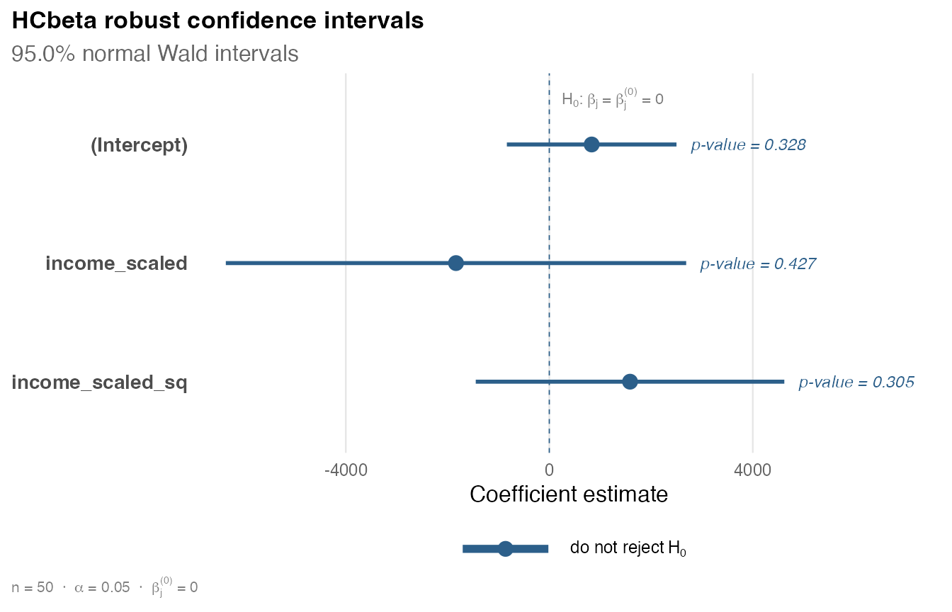
Select one coefficient with parm.
plot(result, parm = "income_scaled_sq")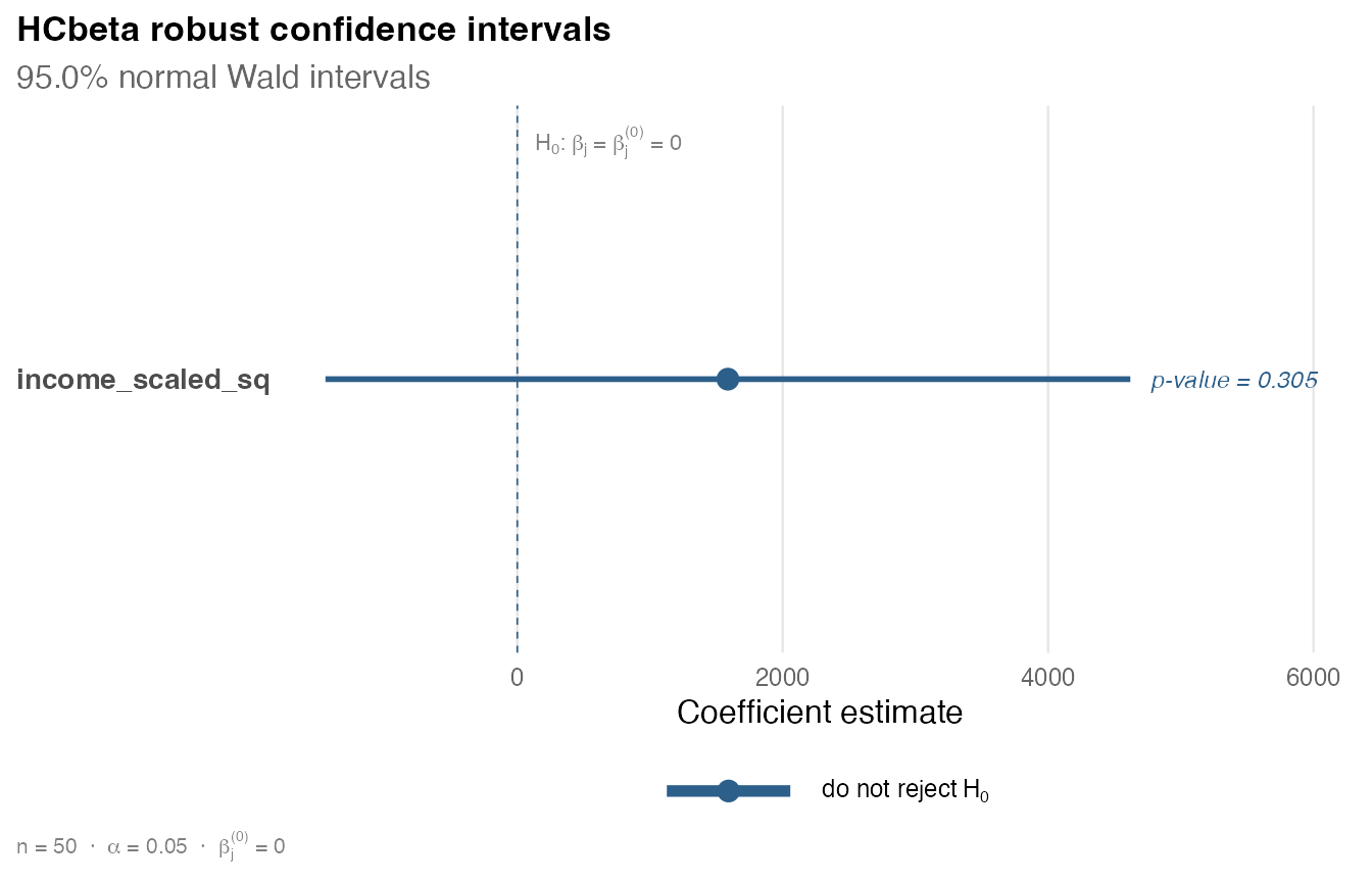
Use plot() on a vcov_hc() object to show
leverage values and HC adjustment factors.
plot(cov_hcbeta)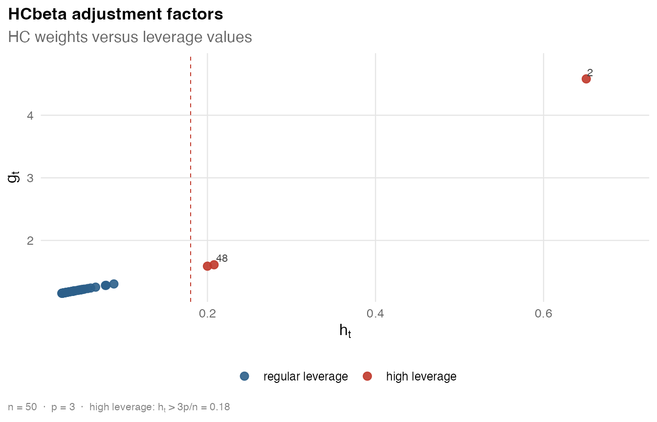
Set label_top to control how many observations with the
largest adjustment factors are labeled.
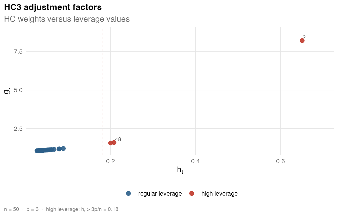
A Small Comparison
The following base R code compares HCbeta and HC3 for the quadratic income coefficient.
test_hcbeta <- tests(result, parm = "income_scaled_sq")
test_hc3 <- tests(result_hc3, parm = "income_scaled_sq")

comparison <- data.frame(
  estimator = c("HCbeta", "HC3"),
  estimate = c(test_hcbeta$estimate, test_hc3$estimate),
  robust_se = c(test_hcbeta$std_error, test_hc3$std_error),
  p_value = c(test_hcbeta$p_value, test_hc3$p_value)
)

comparison
#>   estimator estimate robust_se   p_value
#> 1    HCbeta 1587.042  1547.458 0.3050896
#> 2       HC3 1587.042  1995.242 0.4263730