Pairs bootstrap standard errors and confidence intervals

Computes pairs (case) bootstrap standard errors and confidence intervals for the coefficients of an ordinary least squares model fitted with stats::lm(). The pairs bootstrap resamples the observations \((y_t, x_t)\) with replacement, refits OLS on each resample, and summarizes the resulting sampling distribution of \(\hat\beta\). It makes no assumption about the form of the error variance, so it is a useful empirical reference for the analytic heteroskedasticity-consistent standard errors produced by hcinfer() and vcov_hc().

Usage

boot_pairs(
  object,
  B = 1000L,
  level = 0.95,
  ci_type = c("percentile", "basic", "normal"),
  cores = 1L,
  seed = NULL
)

# S3 method for class 'hcinfer_boot'
print(x, ...)

Arguments

object: An ordinary least squares model fitted by stats::lm(). Weighted fits are not supported.
B: Number of bootstrap replicates. A positive integer; defaults to 1000.
level: Confidence level for the intervals, strictly between 0 and 1. Defaults to 0.95.
ci_type: Interval type: "percentile" (default), "basic", or "normal". See Details.
cores: Number of worker processes. A single number greater than or equal to 1; non-integer values are rounded to the nearest integer. The default 1 runs the replicate fits sequentially. Any value that rounds to 2 or more runs them in parallel with purrr::in_parallel() and the mirai backend, which requires the mirai and carrier packages. Parallelism only speeds up the computation and never changes the numeric result.
seed: Optional single number used to seed the resampling for reproducibility. When supplied, the result is deterministic and independent of the number of cores. Defaults to NULL.
x: An object returned by boot_pairs().
...: Unused.

Value

An object of class hcinfer_boot: a list with the original OLS coefficients, bootstrap std_error, bias, interval endpoints conf_low and conf_high, the settings (level, ci_type, B, B_effective, n_failed, cores, seed), the full replicates matrix (B rows by p columns), and a tidy table tibble with columns term, estimate, bias, std_error, conf_low, and conf_high. Use coef(), vcov(), and confint() to extract components.

Details

For each of B bootstrap replicates, a sample of n row indices is drawn with replacement from 1, ..., n, and OLS is refitted on the resampled rows \((y_{i}, x_{i})\). Writing \(\hat\beta^{*}_{(r)}\) for the estimate on replicate r, the bootstrap standard error of coefficient j is the sample standard deviation of \(\hat\beta^{*}_{1,j}, \ldots, \hat\beta^{*}_{B,j}\).

Three interval types are available through ci_type. Let \(q_\alpha\) denote the empirical \(\alpha\) quantile of the bootstrap replicates for a coefficient, \(\hat\beta_j\) the original estimate, \(s^{*}_j\) the bootstrap standard error, and \(\alpha = 1 - \texttt{level}\). The "percentile" interval is \([q_{\alpha/2}, q_{1-\alpha/2}]\). The "basic" (reverse percentile) interval is \([2\hat\beta_j - q_{1-\alpha/2}, \; 2\hat\beta_j - q_{\alpha/2}]\). The "normal" interval is \(\hat\beta_j \pm z_{1-\alpha/2}\, s^{*}_j\), with \(z\) the standard normal quantile.

Reproducibility. When seed is supplied, all resampling indices are drawn once, sequentially, in the main process under that seed, and the per-replicate fit is deterministic. The results are therefore identical whether the run is sequential or parallel and regardless of the number of cores. The caller's random number generator state is saved and restored, so calling boot_pairs() does not disturb a surrounding random stream. When seed is NULL, the current RNG state is used and results are not reproducible.

Parallelism. The default cores = 1 fits the replicates sequentially. When cores rounds to 2 or more, the deterministic per-replicate fits are distributed with purrr::in_parallel(), which uses the mirai package as its backend. boot_pairs() starts cores daemons for the duration of the call and shuts them down on exit; do not call it while relying on externally configured mirai daemons. Parallelism only speeds up the computation: it never changes the numeric result. It is worthwhile mainly for large B or large n; for small problems the setup overhead can dominate.

Rank-deficient resamples. A resample can be rank deficient (for example when a resample omits the observations that identify a coefficient). Such replicates are dropped, a warning reports how many were dropped, and the summaries use the remaining replicates. The call errors if fewer than two valid replicates remain.

References

Davison, A. C. and Hinkley, D. V. (1997). Bootstrap Methods and their Application. Cambridge University Press. doi:10.1017/CBO9780511802843

Efron, B. and Tibshirani, R. J. (1993). An Introduction to the Bootstrap. Chapman and Hall. doi:10.1201/9780429246593

Examples

schools <- PublicSchools |>
  dplyr::mutate(
    income_scaled = income / 10000,
    income_scaled_sq = income_scaled^2
  )
fit <- lm(expenditure ~ income_scaled + income_scaled_sq, data = schools)

# 1. Fit, inspect, and visualize a reproducible pairs bootstrap.
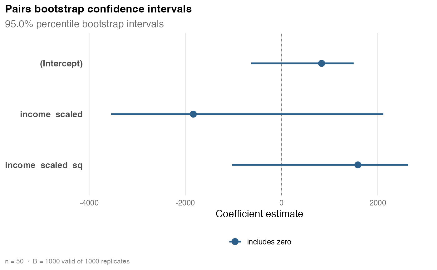
boot <- boot_pairs(fit, B = 1000, seed = 123)
boot
#> 
#> ── 🔎 Pairs bootstrap inference ────────────────────────────────────────────────
#> 📐 Model: `expenditure ~ income_scaled + income_scaled_sq`
#> Observations: 50 | Parameters: 3
#> Replicates: 1000 of 1000 valid | Interval: percentile at 95.0%
#> Execution: sequential | Seed: 123
#> # A tibble: 3 × 5
#>   term             estimate bias   boot_se ci            
#>   <chr>            <chr>    <chr>  <chr>   <chr>         
#> 1 (Intercept)      832.9    -221.1 626.6   [-631.1, 1498]
#> 2 income_scaled    -1834    601.2  1697    [-3545, 2116] 
#> 3 income_scaled_sq 1587     -401.8 1135    [-1027, 2634] 
confint(boot)
#> # A tibble: 3 × 4
#>   term             conf_low conf_high level
#>   <chr>               <dbl>     <dbl> <dbl>
#> 1 (Intercept)         -631.     1498.  0.95
#> 2 income_scaled      -3545.     2116.  0.95
#> 3 income_scaled_sq   -1027.     2634.  0.95
plot(boot)


# 2. Use the bootstrap as an empirical reference for the analytic HC standard
#    errors, side by side in one table.
data.frame(
  term = boot$table$term,
  ols = sqrt(diag(vcov(fit))),
  bootstrap = boot$table$std_error,
  hcbeta = sqrt(diag(vcov(hcinfer(fit, type = "hcbeta")))),
  hc3 = sqrt(diag(vcov(hcinfer(fit, type = "hc3"))))
)
#>                              term      ols bootstrap    hcbeta      hc3
#> (Intercept)           (Intercept) 327.2925  626.6211  850.6572 1095.001
#> income_scaled       income_scaled 828.9855 1696.6723 2308.6541 2975.411
#> income_scaled_sq income_scaled_sq 519.0768 1135.2656 1547.4583 1995.242

# 3. Recompute intervals at a new level and type from the same replicates,
#    without rerunning the bootstrap.
confint(boot, level = 0.99, type = "basic")
#> # A tibble: 3 × 4
#>   term             conf_low conf_high level
#>   <chr>               <dbl>     <dbl> <dbl>
#> 1 (Intercept)          9.28     2546.  0.99
#> 2 income_scaled    -6417.        308.  0.99
#> 3 income_scaled_sq   239.       4625.  0.99
confint(boot, parm = "income_scaled_sq", level = 0.90)
#> # A tibble: 1 × 4
#>   term             conf_low conf_high level
#>   <chr>               <dbl>     <dbl> <dbl>
#> 1 income_scaled_sq    -846.     2526.   0.9

# 4. Larger, parallel run on two cores. Requires the mirai and carrier
#    packages; the numeric result matches a sequential run with the same seed.
# \donttest{
if (requireNamespace("mirai", quietly = TRUE) &&
    requireNamespace("carrier", quietly = TRUE)) {
  boot_par <- boot_pairs(fit, B = 4000, ci_type = "basic", cores = 2, seed = 42)
  boot_par$table
}
#> # A tibble: 3 × 6
#>   term             estimate  bias std_error conf_low conf_high
#>   <chr>               <dbl> <dbl>     <dbl>    <dbl>     <dbl>
#> 1 (Intercept)          833. -213.      625.     182.     2294.
#> 2 income_scaled      -1834.  581.     1688.   -5771.     -160.
#> 3 income_scaled_sq    1587. -389.     1127.     514.     4212.
# }